3 Tree Algorithms

---

Before we move on to the Algorithms, there are few terminologies and assumptions that should be made clear about the distributed network model we consider.

1. The network model is a connected undirected graph - It could be weighted or unweighted

2. Local communication - Nodes can communicated directly(only) with their neighbors through the edges. There are two types of communication.

   • Local unicast - Nodes can send different messages to each of its neighbors (more suitable to wired networks).
   • Local broadcast - Nodes send the same message to all of its neighbors in any step (feature in wireless networks).

3. Synchrony - Two important models can be distinguished based on processor synchronization.

   • Synchronous model - Each processor has an internal clock and the clocks are synchronized. We assume the processor speeds are uniform and each processor takes the same amount of time to perform the same operation. Computation proceeds in lock-step in a series of discrete rounds (time steps). In each round, each processor (node) can do some local (internal) computation and can also send/receive messages. To be concrete, we assume that at the beginning of a round, a node receives messages (if any) from its neighbors via its incident edges.

   • Asynchronous model - No assumptions are made about the internal clocks. We assume that messages arrive in the same order they are sent (FIFO). Algorithms designed for the synchronous model could be transferred to asynchronous model by means of a tool called the synchronizer.

4. Local knowledge - Two models

   • KT0 - (Knowledge of all nodes is restricted Till radius 0) also known as clean network model. Standard model that is typically used. In this model, each node has a port associated with an incident edge (each having a port number). Each node only knows about its own port number and that an edge goes out of it, but nothing about the other endpoint of the edge.

   • KT1 - Here one can assume that the nodes have initial knowledge of their neighbors, especially their IDs.

5. CONGEST vs LOCAL

   • CONGEST - The size of each message sent per round is small, typically of size $O(\log n)$ , where $n$ is the size of the network. This is a reasonable bound as this is at least required to send the unique address of a node. This model captures the inherent bandwidth restriction that is present in real-world networks.

   • LOCAL - There is no restriction on the size of message. This model is useful in focusing on locality issues in distributed computing.

6. Operation - Usually, each node is assumed to operate on the same instance of the algorithm. However, depending on the local information, each node can have its own behavior (due to randomness or unique ID or the information sent by other nodes).

---

Broadcast

Lets look at the following problem:

Given a network $G=(V,E)$ and a source node $s$ , send a message $M$ from $s$ to all nodes in $V$.

Flooding Algorithm:

This algorithm is pretty straightforward. Every vertex $v$ $\ne s$ upon receiving $M$ for the first time, forwards it on every other edge. More like a BFS with visited array, where receiving the message makes the visited flag to be set true and the node no longer sends the message and stops.

Pseudocode:

if v == s then
	send message M to all neighbors and stop
else if M is received for the first time then
	send M to all neighbors and stop

Analysis:

Claim:

The flooding algorithm is correct i.e., all nodes eventually receive the message from the source node. The message complexity is $\Theta (|E|)$ and the time complexity is $D$ , where $D$ is the diameter of $G$.

Proof:

Let $v$ be any node. We use induction on $t$ to show that after $t$ time units, the message has already reached every vertex in ${\mathrm{ball}}_G(s,t)$ .

• Base case: At $t=0$ this is trivially true.
• Induction Step: We assume the hypothesis is true at time $t$. It follows at time $t+1$ , all neighbors of nodes at distance $t$ , which are at distance $t+1$ , will receive the message.

The message complexity follows from the fact that each edge delivers the message at least once and at most twice (one in each direction).

The time complexity is clearly bounded by the diameter, which is the maximum distance between any two nodes in $G$.

Lower bound for Broadcast:

Claim:

Any distributed algorithm for broadcast has a message complexity of $\Omega (n)$ and time complexity of $\Omega (D)$.

Proof:

• Message Complexity: Every node has to receive the message so at least $n-1$ messages are needed. Note that this is not a tight lower bound for broadcast.
• Time Complexity: For any source node $s$ , there exists a node $u$ which is at a distance of at least $\Omega (D)$ from $s$. Note that this is a tight lower bound for broadcast.

Tree Broadcast:

A spanning tree-based broadcast from a source node $s$ proceeds as follows. The root $s$ sends the message to its neighbors. When a node $v$ receives the messages for the first time, it forwards it along the tree edges only except to the parent node. If $v$ receives the message again, it ignores as usual.

Claim:

Given a graph $G$ with spanning tree $T$ rooted at $s$, the message complexity of broadcast from $s$ is $n-1$ and time complexity is $\mathrm{height}(T)$ .

This is just substitution of $m=n-1,D\ge \mathrm{height}(T)$ in the previous results.

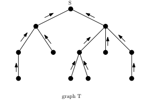
Convergecast

This can be viewed as the opposite to broadcast, where the all the nodes send the information to the root of a spanning tree in an upwards fashion.

Let $T$ be a spanning tree rooted at node $r$ . Let’s say we each node has a value $a_v$ and we need the sum of values of the network. Then we can run the following algorithm. Start from the leaf nodes. In the first round, each leaf node sends its value to the parent. The parent nodes sum up all the values it receives and adds its own value as well. This value is sent up when it gets information from all the children This process terminates at the root $r$. The time taken $O(\mathrm{height}(T))$ .

Consider the flooding algorithm. Suppose the source wants to know when the algorithm terminated. First, the flooding can be used to construct a spanning tree rooted at the source. Let $T$ be the spanning tree. Each leaf node in the tree will send an echo message to its parent. Each internal node, when it receives from all the children will send an echo message to the parent. Once the root receives the echo messages from all its children, it will know that the broadcast algorithm has terminated successfully.

Pipelining:

Consider the following problem: Each node has a list of $k$ values i.e. each node has values $[a_i(1),a_i(2),...,a_i(k)]$ , and the goal is to compute the list of component wise sums

$$\left[\sum _{i=1}^n{a}_i(1),\sum _{i=1}^n{a}_i(2),...,\sum _{i=1}^n{a}_i(k)\right]$$

at some source $s$ .

Instead of a straightforward algorithm of performing convergecast $k$ times for each element in the list ($O(k\cdot \mathrm{height}(T))$ time), we can do much better using something called pipelining.

Each node when it receives the value send the aggregated values component by component to their respective parent. More formally, for the first $k$ rounds, the leaf nodes will send the list values one by one. An intermediate node $v$ would receive all the values of $j$th component in the round $j+\mathrm{height}(v)$ . At this time, it will send the aggregated values along with its value to its parent. Using an inductive argument, it could be shown that the total number of rounds would be $O(k+\mathrm{height}(T))$ .

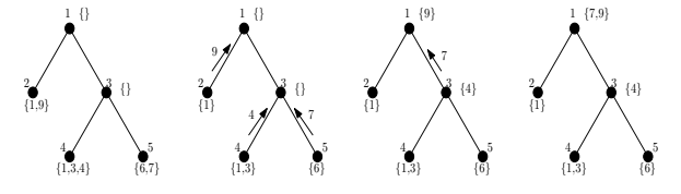
Upcast

Consider the following problem: We are given $k$ items distributed arbitrarily on the nodes of a network $G=(V,E)$. A node can have zero , one or more items. We would like to collect all these items at a node $s$ $\in V$ . Assume that item size is small, has a unique ID and can be represented in $O(\log n)$ bits.

We cannot do convergecast as aggregating items isn’t possible. Instead we modify the convergecast and do it individually for each item, which would be inefficient and would take $O(k\cdot \mathrm{height}(T))$ time.

Consider the following algorithm - At any round, each node does the following: Among the set of items that it currently has, send the item with highest ID (highest priority) to its parent. The sent item is removed from the set of items it currently has. The main idea of this algorithm is to use the ID to break ties. This is useful while analyzing the algorithm.

Claim:

The above algorithm upcasts all the items to the root and takes $O(k+\mathrm{height}(T))$ time.

Proof:

Idea: Note that the highest priority element is never delayed in any round i.e., it is sent to the root in $O(\mathrm{height}(T))$ time to the root. The second highest element, can be delayed only by the highest element, and that too only once. Let $x$ be the highest priority element and $y$ is the second highest priority element. The previous statement is true since once $y$ gets delayed and $x$ moves up, there is no other element to delay both $x$ and $y$, as well as $x$ can’t delay as it has moved up already.

Consider the $j$-th highest priority element. It can possibly delayed by the items that are at higher priority than this element. Let $j^{\prime }$ be the priority of the element of the lowest priority that delays $j$-th priority element. Note that once this happens, it is never delayed again by $j^{\prime }$ and any further delay can only be attributed to an item that is ranked higher than $j^{\prime }$, let’s say $j^{\prime \prime }$. This is because $j^{\prime \prime }$ can delay $j^{\prime }$ and make $j$ catch up with $j^{\prime }$ , This would incur an additional delay, but that delay could be attributed to $j^{\prime \prime }$ . Thus the $k$-th element would at most incur a delay of $k$.

Downcast

Inverse problem of upcast. Instead of collecting things to a single node, we distribute things from a single node to all nodes. We can do this by an algorithm very similar to the one used in upcast. When sending message to neighbors, choose the ID with the lowest priority and send it. This can be done in $O(k+\mathrm{height}(T))$ time.

BFS Spanning Tree

The Flooding algorithm could be modified to convert the network into a breadth-first spanning tree only network. In other words, once the algorithm terminates, each node will be aware of its parent as well its children in the spanning tree. Note that the root node will not have any parent and leaf nodes won’t have any children.

Distributed BFS Tree construction:

Source node $s$ sends an invite message inviting its neighbors to be its children. When a node $v$ receives an invite message from one or more neighbors for the first time, it will respond exactly to one such invite message. It does by sending an accept message to its parent. Any invite message in the later rounds is ignored. Very similar to visited array concept used in graph traversal.

Pseudocode:

if v == s then
	send "invite" message to all neighbors
	designate all neighbors as children
else if when "invite" message is received for the first time, then
	send "accept" to exactly one neighbor p , make p as the parent.
	send "invite" message to all neighbors except p.
	when "accept" message is received from any neighbor u, make u as a child.

Analysis:

Correctness analysis can be done using induction. Message and Time complexity is asymptotically equivalent to the message complexity of Flooding i.e., $O(|E|),O(D)$.

Termination Detection:

This is a global knowledge i.e., requires knowledge about status of all the nodes in the network. As we saw in the convergecast, each node can just echo back once all its children has echoed back. As for the leaf nodes, leaf nodes will echo back immediately and leaf nodes can self identify themselves by identifying that no accept message has arrived in the subsequent round. Once the root node receives the echo from all its children, a broadcast can be done to all the other nodes, so that the termination message is spread over the network.

Information Spreading

Given a network $G=(V,E)$ of $n$ nodes and $m$ edges, and a set of $k$ tokens arbitrarily distributed among the $n$ nodes, we need to disseminate the $k$ tokens to all the nodes. This problem can be viewed as a generalization of upcast, here we need to send it to all nodes instead of the root node only. One application of this is to acquire global knowledge of the network, when every node wants to know the global topology.

Consider the following algorithm: Find a BFS tree. Then upcast all $k$ items to the root of the tree. Then we downcast the items to all the nodes. Overall time complexity of this algorithm would be $O(D)+O(D+k)+O(D+k)=O(D+k)$.

For the message complexity, it is clear that $\Omega (nk)$ is a lower bound, as only one message is passed each round and each node has to get $k$ messages. Overall message complexity of this algorithm would be $O(m)+O(kD)+O(nk)=O(m+nk)$ .

Exercises

Will be added soon